Table of Contents
Working with Maps
Mapping allows you to transform the data in one variable (defined by one or more informants) into another variable (with different informants), based on a defined map structure. Here we will outline the instances that mapping is used.
Map Tool
The map tool is the main way to map the elements in one variable according to a map into the elements in another variable. There are three main types of maps that the map tool uses: full matrix, dimension and index. Examples and uses of these mapping types are explored below.
Full Matrix Mapping
The full matrix map is used to map a complete set of elements to another set of the elements and is commonly used to aggregate elements into classes and transfer data from one set of elements to another set of elements.
Aggregation into classes
This is a common use of the map tool. Using the example below the map tool is used to aggregate populations by age into several status classes based on the data in the image below.

The supporting tool script code for building the informants and importing data from the data source can be found here.
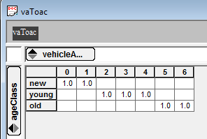
The first step is to create the map indicating how the elements relate to each other. For this example ages 0 to 1 are classified as new, ages 2 to 4 are classified as young and ages 5 to 6 are classified as old.
local vaToac[ageClass,vehicleAge] = create (; dim=ageClass, dim=vehicleAge, format=mapping, \
	0 -> new, \
	1 -> new, \
	2 -> young, \
	3 -> young, \
	4 -> young, \
	5 -> old, \
	6 -> old)

table (vaToac[ageClass,vehicleAge])
By using the table tool you can see the matrix that has been constructed in the vaToac[ageClass,vehicleAge] variable and how one element is mapped to the other (by default Table hides all zero values).
local vehicleClass[vType,ac] = map (vehicles[vType,va], vaToac[ageClass,vehicleAge])

table (vehicleClass[vType,ac])
As you can see in the following table every point for ages 0 to 1 is aggregated and classified as “new”, while ages 2 to 4 aggregated and classified as “young” and ages 5 to 6 are aggregated and classified as “old”
Element mapping
One reason for creating a map is because the element names in the source data do not match the elements in your model. This map can be as simple as passing the source data from one element to another, passing data from one element to many elements in the model on a one-to-one basis or passing data from one source element to many elements in the model based on specified splits.
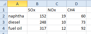
All of the following element mapping examples refer to the data found in the image below.
The supporting tool script code for building the informants and importing data from the data source can be found here.
one element to another element
Mapping source data from one element to another is useful when the element names in your database do not match the element names in your model.
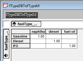
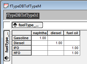
The first step is to create the map indicating how the elements relate to each other. For this example naphtha is mapped to Gasoline, diesel is mapped to Diesel and fuel oil is mapped to IFO.
local fTypeDBTofTypeM[fTypeM,fTypeDB] = create (; dim=fuelType_model, dim=fuelType_DB, format=mapping, \
	"naphtha" -> "Gasoline", \
	"diesel" -> "Diesel", \
	"fuel oil" -> "IFO")

table (fTypeDBTofTypeM[fTypeM,fTypeDB])
By using the table tool you can see the map that has been constructed in the fTypeDBTofTypeM[fTypeM,fTypeDB] variable and how one element is mapped to the other (by default Table hides all zero values).
local fuelEm_model[fTypeM,em] = map (fuelEm_DB[fTypeDB,em], fTypeDBTofTypeM[fTypeM,fTypeDB])

table (fuelEm_model[fTypeM,em])
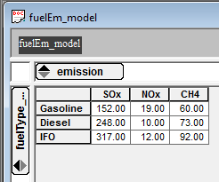
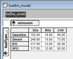
The table below displays the results of the map tool, see how the row names now correspond to the elements in the fuelType_model dimension.
one element to many elements
This is useful when the granularity of your elements is finer than the elements provided in your source data. For example your source data contains emissions data for fuel oil however your model captures the various grades of fuel oil as seen below.
The supporting tool script code for building the informants and importing data from the data source can be found here.
As in the previous example the first step is to create the map indicating how the elements relate to each other. For this example naphtha is mapped to Gasoline, diesel is mapped to Diesel and fuel oil is mapped to both IFO and HFO.
local fTypeDBTofTypeM[fTypeM,fTypeDB] = create (; dim=fuelType_model, dim=fuelType_DB, format=mapping, \
	"naphtha" -> "Gasoline", \
	"diesel" -> "Diesel", \
	"fuel oil" -> "IFO, HFO")

table (fTypeDBTofTypeM[fTypeM,fTypeDB])
By using the table tool you can see the matrix that has been constructed in the fTypeDBTofTypeM[fTypeM,fTypeDB] variable and how one element is mapped to the other (by default Table hides all zero values).
local fuelEm_model[fTypeM,em] = map (fuelEm_DB[fTypeDB,em], fTypeDBTofTypeM[fTypeM,fTypeDB])

table (fuelEm_model[fTypeM,em])
The table below displays the results of the map tool, see how the row names now correspond to the elements in the fuelType_model dimension and how the values have been duplicated for both IFO and HFO.
one element to many elements using splits
The above exmaple simply copied the data for fuel oil in the database to both the IFO and HFO elements in the model. However there may be times that you want the data to be split in some way between the elements. Unfortunately fractions can not be specified when using the “goes into” or “→” parameter. Therefore you must use the following method to specify how the data is split between two or more elements.
The supporting tool script code for building the informants and importing data from the data source can be found here.
As in the previous example the first step is to create the map indicating how the elements relate to each other. This map is created differently than the previous examples. In this case you need to manually populated that map by using the method outlined below.
local fTypeDBTofTypeM[fTypeM,fTypeDB] = create (; dim=fuelType_model, dim=fuelType_DB, \
	data="1 0 0 0 1 0 0 0 0.5 0 0 0.5")

table (fTypeDBTofTypeM[fTypeM,fTypeDB])
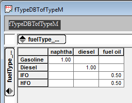
By using the table tool you can see the map that you have manually constructed in the fTypeDBTofTypeM[fTypeM,fTypeDB] variable and how this relates the syntax found in the code above. (by default Table hides all zero values).
local fuelEm_model[fTypeM,em] = map (fuelEm_DB[fTypeDB,em], fTypeDBTofTypeM[fTypeM,fTypeDB])

table (fuelEm_model[fTypeM,em])
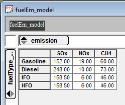
The table below displays the results of the map tool, see how the row names now correspond to the elements in the fuelType_model dimension and how the values have been multiplied by 0.5 for both IFO and HFO.
Dimension Mapping
The dimension map is a quick method that is used to map a set of elements to another set of the elements. However for a dimension map to work the element names in both informants need to be spelled exactly the same. This method is useful for mapping data from a set of elements to a subset of those elements as seen in the example below.
The supporting tool script code for building the informants and importing data from the data source in the table above can be found here.
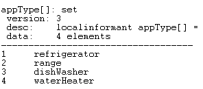
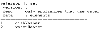
Unlike the full matrix method, dimension mapping does not require the creation of a map template because the mapping is based on element names. Using the display tool below we can what elements are in appType and waterApp informants to ensure that dimension mapping is possible.
display (appType[], waterApp[])
We can see that both informant contain the elements dishWasher and waterHeater so we can proceed with the dimension mapping of these elements as follows.
local waterAppliances[wApp,t] = map (appliance[aType,t]; appType->waterApp)

table (waterAppliances[wApp,t])
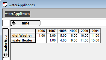
The table below displays the results of the map tool, see how the variable waterApplicanes[wApp,t] now contains data for only the dishWasher and waterHeater elements
Index Mapping
Index mapping allows you to map the right-most dimension of a variable onto the new dimension. This is the most difficult method to use because you need to know the position in the array or index number of the element(s) you are interested in mapping as well as the order of your informants.
This example demonstrates how you can take a subsection of elements from the data in the table below and map them into the complete set using both the one to one and many to one mapping parameters.
The supporting tool script code for building the informants and importing data from the data source can be found here.
As in the full matrix method we need to first create a map indicating how the elements relate to each other. The data parameter in the create tool indicates the position in the array or the index number that we will be mapping to. Also notice that the map tool requires you to specify the new dimension
local mapPriaire[pp] = create (; dim=prairieProv, dataType=integer, data="4 5 6")

regions_a[t,r] = map ( prairieData[t,pp], mapPriaire[pp]; mapping=oneToOne, newDim=region)

table (regions_a[t,r])
As you can see in the following table data for Alberta, British Columbia and Saskatchewan has been individually mapped into the variable regions_a[t,r].
As with the one to one mapping the map indicating how the elements related to each other needs to be created. However notice how the index numbers are all pointing to the same position in the array.
local mapAtlantic[ap] = create (; dim=atlanticProv, dataType=integer, data="1 1 1 1")

regions_b[t,r] = map ( atlanticData[t,ap], mapAtlantic[ap]; mapping=manyToOne, newDim=region)

table (regions_b[t,r])
In contrast to the one to one example all of the values for the Atlantic provinces have been aggregated and mapped into the Atlantic element in the regions_b[t,r] variable.
Mapcat Tool
A category is a useful way of grouping elements into meaningfull collections. By categorizing related elements together you can create elements that are more descriptive while also reducing the number of elements you are carrying through your model.
The mapcat tool can also be used for aggregating elements into classes or groups. The example below uses the data found in the following table to use the categorization as a map to transform the population data for each province to a region class while aggregating over each province to get the total population in each region.
The supporting tool script code for building the informants and importing data above can be found here.
The mapping template for a category is held in the category itself. As you can see in the code below the provinces is the group place holder and the locations are members of the province and they are related to each based on a relationship provided by the modeler.
localinformant locProv[l->p] = create (; object=category, groups=location, members=province, \
	"west"="Alberta", \
	"west"="British Columbia",\
	"east"="Newfoundland",\
	"east"="Nova Scotia",\
	"central"="Ontario",\
	"east"="PEI")
This categorization or map can then be applied using the mapcat tool below to bring the elements together in the category.
local provLoc_Cat[l->p] = mapcat (provinceData[p]; category=locProv)

table (provLoc_Cat[l->p])
See how the province and location informants have been categorized into the provLoc category.
Now we can use the mapcat tool again, but this time we will be splitting the category back up into the respective group and members.
local regions[l,p] = mapcat (provLoc_Cat[l->p])

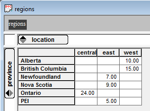
table (regions[l,p])
See how we have now created a two dimensional array from a data set that only had one dimension.
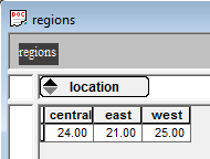
We can now sum up the provinces dimension to get the total population for each region as seen in the table below.
local regions_sum[l] = sum (regions[l,p]; \
	dim=province)

table (regions_sum[l])
This process has been broken down inorder to see how the transformation occurs, however there is no need to take this many steps. This process can be done on one line by combining the two mapcat and sum tool commands as follows:
local regions[l] = sum (mapcat (mapcat (provinceData[p]; \
	category=provLoc); \
	dim=provLoc); \
	dim=province)

